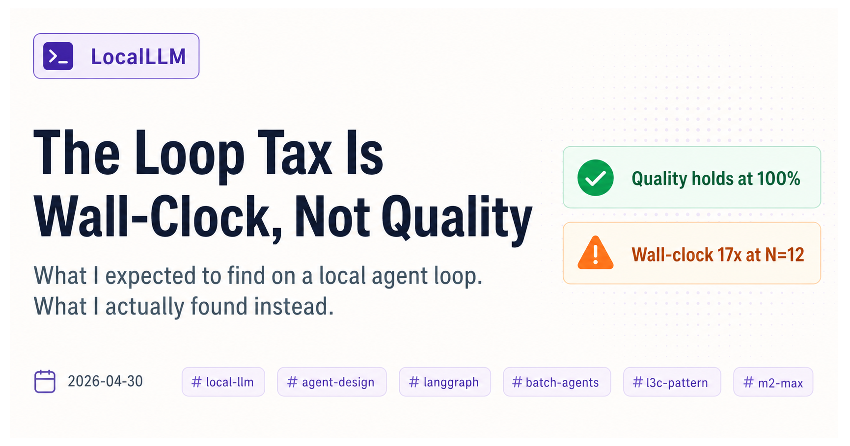

The Loop Tax Is Wall-Clock, Not Quality
I went looking for the loop tax. The premise was familiar: production agents trail their eval scores because the loop wears them down. I built a four-branch falsification on a Mac Studio M2 Max with gemma4:26b (A4B MoE, Q4_K_M) and pushed the iteration count to N=15 with explicit factor isolation between depth and state size to nail down the cause.
The cliff didn’t surface. Quality stayed at 100% across every cell.
What did surface, with numbers, was a wall-clock divergence between branch designs that’s just as practical: the same model on the same task pays a ~17x TTFT tax under a full-context loop versus a flat profile under a batch + state file design. This post is what the falsification actually returned, and why I think the wall-clock side is the live story for local agents.
This is the third post in what I’m starting to think of as a “Local LLM Ops” series. The earlier two covered the system axis: where the same model behaves differently across runtimes, and where memory accounting on Apple Silicon misleads. This one is about the design / temporal axis.
What I expected to find
The shorthand version: production agents trail their eval scores because eval is clean single-shot while production is the loop layer where coupling between turns brings the ceiling back. The trope I kept seeing on dev Twitter was an “iteration 6-7 ceiling on local 27B/35B agent loops.” Local models with smaller context budgets feel the tax sooner, the argument goes, because coupled noise from prior turns eats a bigger fraction of working space.
I went into this expecting the bench to surface that ceiling at N≈9 on gemma4:26b, ideally with branch C (depth grown, state capped) and branch D (depth held, state padding grown) splitting depth-driven failure from coupling-driven failure cleanly. With four branches, two runtimes, and N up to 15, the picture should have been unambiguous.
It was unambiguous. Just not in the direction I expected.
The four-branch design
| Branch | What it does | What it isolates |
|---|---|---|
| A | Full-context loop. All conversation history accumulates in messages. |
Depth and state size, confounded |
| B | Batch + cumulative state file. Each turn reads a state file, emits the new full state, atomic-rename writes back. | Same confounding as A but via state file (production-shape) |
| C | Cap state size + grow depth. State file holds at most cap_size=3 most-recent entries; count tracks cumulative total. |
Depth-driven failure, with state size held |
| D | Hold depth + grow state padding. Depth fixed at N=3; state pre-populated with padding_size synthetic entries. |
Coupling-driven failure, with depth held |
Branches A and B let depth and state size grow together (linearly confounded). Branches C and D each pin one axis and grow the other, so a cliff in C points to depth as the cause, and a cliff in D points to state-size coupling. This 2x2 structure was the centerpiece of the falsification.
The task itself was an iterative research log update: each turn supplies one new entry; the model must emit the complete updated log as schema-conformant JSON, sorted newest-first, wrapped in a json fenced block. Strict schema, every turn, every branch.
What I measured
Per turn, the bench logs:
valid_json— fenced JSON parses successfullyschema_ok—logis a list of dictscount_match—countfield matches expected cumulative totalentries_complete—log[]length matches expectedsort_correct— entries are sorted newest-firstall_pass— all five flags truecond_pass—P(turn t passes | turn t-1 passed), the conditional pass rate that would surface a tail-clustered failure modecontext_tokens_estimate— char-based proxystate_file_bytes— actual size of the state file fed back into the next turndecode_tps,ttft_ms— runtime-level signals
Conditions:
- Models:
gemma4:26b(Ollama-distributed blob) on the Ollama side, andgemma-4-26B-A4B-it(upstreamggml-orgHF GGUF, Q4_K_M) on the llama.cpp side. These are different artifacts; the Ollama-distributed Gemma 4 blob does not load on llama.cpp 8940 (see previous post). Within-runtime branch comparisons are clean; cross-runtime numbers mix runtime and packaging - Runtimes: Ollama (default), llama.cpp (Homebrew formula 8940, post-tag
b6869) - N values: A/B at 1, 3, 6, 9, 12; C at 1, 3, 6, 9, 12, 15; D at depth=3 with
padding_size∈ {1, 3, 6, 9} - 5 runs per cell, 40 cells total
- Sampling fixed across all branches:
temperature=0.2, top_p=0.95, top_k=40, seed=42
What didn’t show up: the quality cliff
The result that mattered most for the original thesis is also the simplest to state.
all_pass_rate was 100% across every one of the 40 cells.
Branch A at N=12 with full conversation history. Branch C at N=15 with the depth axis pinned. Branch D with padding_size=9 synthetic entries inflating the state. gemma4:26b produced schema-correct, count-correct, sort-correct output, every turn, every run. cond_pass was 100% wherever it could be defined.
That makes the falsification scoreboard read like this:
| H | Description | Status |
|---|---|---|
| H1 | Branch A all_pass_rate decreases monotonically with N |
Rejected (100% through N=12) |
| H2 | Branch B stays flat with N | Supported, trivially (everything is 100%) |
| H3 | A-vs-B gap widens with N | Rejected (no gap, both 100%) |
| H4 | Branch C cliff implies depth-driven failure | Rejected (no cliff at N=15) |
| H5 | Branch D cliff implies coupling-driven failure | Rejected (no cliff at padding=9) |
A negative result on a falsification of the form “X causes Y” is informative: on this task, on this model, in this scale of loop, the loop tax does not show up as a quality cliff. That isn’t the same as saying it doesn’t exist. It is saying that the place I expected it to live, on a model that is well-matched to the task, is not where the failure mode hides.
What did show up: wall-clock divergence
The structural difference between branches showed up cleanly on TTFT.
Branch A — full-context loop, llama.cpp, N=12
| turn | ctx_tok | TTFT (ms) |
|---|---|---|
| 1 | 161 | 60 |
| 3 | 406 | 126 |
| 6 | 1053 | 511 |
| 9 | 2034 | 763 |
| 12 | 3347 | 1046 |
Turn 1 → turn 12: TTFT grew from 60 ms to 1046 ms (17.4x). Context tokens grew from 161 to 3347 (20.8x). Decode throughput drifted slightly, from 67.9 t/s to 62.8 t/s.
Branch C — cap state at 3, llama.cpp, N=15
| turn | ctx_tok | state_bytes | TTFT (ms) |
|---|---|---|---|
| 1 | 256 | 68 | 122 |
| 3 | 332 | 375 | 107 |
| 6 | 367 | 517 | 103 |
| 9 | 368 | 519 | 103 |
| 12 | 364 | 510 | 104 |
| 15 | 365 | 510 | 100 |
Turn 1 → turn 15: TTFT essentially flat at ~100-122 ms. Context tokens stop climbing once the cap takes effect (~turn 4). Decode throughput stable at ~65.5 t/s (range 65.4–66.3) across all 15 turns.
Branch B — batch + cumulative state, llama.cpp, N=9
| turn | ctx_tok | TTFT (ms) |
|---|---|---|
| 1 | 181 | 124 |
| 5 | 331 | 109 |
| 9 | 480 | 165 |
State accumulates entries linearly so ctx_tokens does grow, but TTFT stays in the ~85–290 ms range over 9 turns, mostly clustered in the 100–200 band with a turn-2 outlier near 290 ms.
Branch D — hold depth at 3, llama.cpp, padding sweep
| padding_size | turn 1 ctx_tok | turn 1 state_bytes | turn 1 TTFT (ms) |
|---|---|---|---|
| 1 | 215 | 206 | 156 |
| 3 | 293 | 515 | 309 |
| 6 | 403 | 958 | 355 |
| 9 | 512 | 1391 | 266 |
The cold-start TTFT does scale with state size, roughly, though noise is visible (the padding=9 row is lower than padding=6 once). Across runs, the mid-band tracks state size; once the conversation enters its (short) steady state, TTFT settles toward the flat profile branch C shows.
The pattern
Same task, same prompt, same sampling, same model family, same correctness — branch is the only variable:
- Branch A pays ~17x TTFT by turn 12, because every turn re-reads the entire growing history.
- Branch C is flat because the cap holds the relevant context constant.
- Branch B sits between them, growing slowly because the state file grows linearly with N but doesn’t include the model’s own past output verbatim.
- Branch D shows the cold-start cost of injecting a larger state file at the start, then settles.
The quality of the produced JSON does not change. The latency a user observes for the same task does change, by an order of magnitude.
Why this still matters even without a quality cliff
Two reads of the negative result are worth holding side by side.
The conservative read. I picked a task that turned out to be well-matched to gemma4:26b at this scale. A more challenging task, a smaller model, or a longer loop might still surface the quality cliff I expected. The way to find out is to push more axes — more entries, more permissive schema, time-to-first-success at temperature 0, smaller models — until the model actually begins to fail. That’s the natural next bench.
The structural read. Even when quality is bulletproof, the choice of branch shape determines whether the loop pays a 17x wall-clock cost or a flat one. Eval scores can tell you the model is fine. They cannot tell you the loop is fine, because eval is a single shot. Production tells you the loop is fine on quality and not on latency, which is the exact split between the two reads above.
For a local 27B/35B running on a Mac, that gap is the thing a user experiences. Hitting “go” on an agent that streams over twelve turns is the difference between roughly a second per first token and roughly a hundred milliseconds per first token. That difference compounds. Multi-turn agent UX on this stack (27B-class MoE, Apple Silicon, llama.cpp/Ollama) is dominated by the first-token latency tax under shape-A loops, not by output throughput, and not by output quality.
The L3c sequel — agent loop edition
The first L3c post argued that, for any individual skill, deterministic structural work belongs in code (L3c), not in the LLM’s prompt. This run is the same argument extended one level up.
For an agent loop the question is: where does state live between turns? If it lives in the conversation, the model re-reads its own past output every turn and pays the prefix cost. If it lives in a file outside the conversation, the model sees a freshly serialized snapshot and a single new piece of work. Same correctness. Different wall-clock.
Branch C pushes this further: the state file itself is bounded. The model’s effective context is decoupled from the iteration count. The wall-clock floor is set by the state size and the system prompt, and it stays there.
Three kinds of work, three placements:
- Judgment about what to do next — the model.
- Constraint about what valid output looks like — the prompt.
- Persistence and pruning of state across turns — code, atomically, outside the model.
The third one is what changed branch A’s 17x TTFT growth into branch C’s flat profile, while the model itself produced identical output quality.
What this post does not cover
- Tasks that require prior conversational context. Some agents are conversational by design; the shape-A picture is the right one for those. The argument here is about agents whose job is to advance state, not to maintain a dialogue.
- A quality cliff that this task didn’t surface. A more complex task, a weaker model, or a longer loop may still produce the failure mode I was looking for. This run does not rule it out.
- Time-to-first-success at temperature 0. A retry-budget metric that the conversation around this work surfaced as the next obvious cut. Not implemented in this run; on the list as a follow-up.
- NVIDIA / Linux setups. Different runtime path, different memory accounting, different latency profile. Not measured here.
- Frontier API models. The wall-clock numbers above are for a 26B-A4B MoE on Apple Silicon. Above that scale, the same shapes still apply, but the magnitudes change.
Closing
The cliff I was looking for didn’t show up. The cliff I wasn’t looking for did.
Eval can tell you the model is fine on a single shot. The loop tax that does show up on local hardware is not a quality cliff at iteration N; it is a wall-clock cost that scales with how much past output you re-read every turn. Quality is the same across the four shapes. Latency is not.
The way to absorb that cost is the same shape the L3c Pattern points at: keep state out of the conversation. Cap it where you can. Atomic-write it. Run the model on the smallest narrow context that contains the next decision, and only the next decision.
My logs, my setup, my falsification. Verify on your own box.
Source material: test_f_iteration_drift.py runs on 2026-04-30, Mac Studio M2 Max 64 GB, Homebrew llama.cpp formula 8940 (post-tag b6869), Ollama latest stable. Raw test records in benchmarks/results/test_f_*.json, aggregated in drafts/results_loop_tax.md. 40 cells × 5 runs × up to 15 turns; per-turn flags, conditional pass rate, state-file bytes, TTFT, and decode tps logged for every turn.